Computing and plotting π with Gonum and a zest of Monte Carlo
Today we will see how we can compute π with a technique called Monte Carlo.
Wikipedia, the ultimate source of truth in the (known) universe has this to say about Monte Carlo:
Monte Carlo methods (or Monte Carlo experiments) are a broad class of computational algorithms that rely on repeated random sampling to obtain numerical results. (…) Monte Carlo methods are mainly used in three distinct problem classes: optimization, numerical integration, and generating draws from a probability distribution.
In other words, the Monte Carlo method is a numerical technique using random numbers.
With Monte Carlo integration, we can estimate the value of an integral:
- take the function value at random points
- the area (or volume) times the average function value estimates the integral.
With Monte Carlo simulation, we can predict an expected measurement:
- an experimental measurement is split into a sequence of random processes
- use random numbers to decide which processes happen
- tabulate the values to estimate the expected probability density function (PDF) for the experiment.
In High Energy Physics (HEP) – but also in many other scientific domains – the Monte Carlo method is used to model a phenomenon, to create a simulation of a given process (and perhaps compare that simulation with measurements of the real world.) In HEP, we have very detailed simulation programs (like Geant4 that models interactions of particles with matter using all our knowledge of particle physics) and fast simulation programs (like Delphes (C++) or fads (in Go)) that very coarsely model physics. But before being able to write a HEP detector simulation, we need to know how to generate random numbers in Go.
Generating random numbers
The Go standard library provides the building blocks for implementing Monte Carlo techniques, via the math/rand package.
math/rand exposes the rand.Rand type, a source of (pseudo) random numbers.
With rand.Rand, one can:
- generate random numbers following a flat, uniform distribution between
[0, 1)withFloat32()orFloat64(); - generate random numbers following a standard normal distribution (of mean 0 and standard deviation 1) with
NormFloat64(); - and generate random numbers following an exponential distribution with
ExpFloat64.
If you need other distributions, have a look at Gonum’s gonum/stat/distuv.
math/rand exposes convenience functions (Float32, Float64, ExpFloat64, …) that share a global rand.Rand value, the “default” source of (pseudo) random numbers.
These convenience functions are safe to be used from multiple goroutines concurrently, but this may generate lock contention.
It’s probably a good idea in your libraries to not rely on these convenience functions and instead provide a way to use local rand.Rand values, especially if you want to be able to change the seed of these rand.Rand values.
Let’s see how we can generate random numbers with "math/rand":
|
|
Running this program gives:
1 2 3 4 5 6 7 8 9 10 11 |
$> go run ./mc-0.go 0.8487305991992138 0.6451080292174168 0.7382079884862905 0.31522206779732853 0.057001989921077224 0.9672449323010088 0.6139541710075446 0.01505990819189991 0.13361969083044145 0.5118319569473198 |
OK. Does this seem flat to you? Not sure…
Let’s modify our program to better visualize the random data. We’ll use a histogram and the go-hep.org/x/hep/hbook and go-hep.org/x/hep/hplot packages to (respectively) create histograms and display them.
Note: hplot is a package built on top of the gonum.org/v1/plot package, but with a few HEP-oriented customization.
You can use gonum.org/v1/plot directly if you so choose or prefer.
|
|
We’ve increased the number of random numbers to generate to get a better idea of how the random number generator behaves, and disabled the printing of the values.
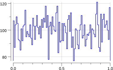
We first create a 1-dimensional histogram huni with 100 bins from 0 to 1.
Then we fill it with the value r and an associated weight (here, the weight is just 1.)
Finally, we just plot (or rather, save) the histogram into the file "uniform.png" with the plot(...) function:
|
|
Running the code creates a uniform.png file:
1
|
$> go run ./mc-1.go |

Indeed, that looks rather flat.
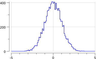
So far, so good. Let’s add a new distribution: the standard normal distribution.
|
|
Running the code creates the following new plot:
1
|
$> go run ./mc-2.go |

Note that this has slightly changed the previous "uniform.png" plot: we are sharing the source of random numbers between the 2 histograms.
The sequence of random numbers is exactly the same than before (modulo the fact that now we generate -at least- twice the number than previously) but they are not associated to the same histograms.
OK, this does generate a gaussian.
But what if we want to generate a gaussian with a mean other than 0 and/or a standard deviation other than 1 ?
The math/rand.NormFloat64 documentation kindly tells us how to achieve this:
“To produce a different normal distribution, callers can adjust the output using:
sample = NormFloat64() * desiredStdDev + desiredMean“
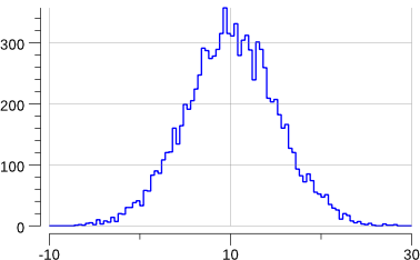
Let’s try to generate a gaussian of mean 10 and standard deviation 2.
We’ll have to change a bit the definition of our histogram:
|
|
Running the program gives:
1 2 3 |
$> go run mc-3.go gauss: mean= 10.105225624460644 gauss: std-dev= 5.048629091912316 +/- 0.05048629091912316 |

Ok, so now we know how to generate random numbers that follow some distribution. How do we evaluate π with that?
Approximating π using a Monte Carlo technique
Consider a circle inscribed in a unit square:
- the unit square has an area of
d^2 = (2r)^2 = 4r^2, (wheredis the diameter of the circle andrits radius) - the unit circle has an area of
π.r^2.
The ratio of these two areas is thus area(circle)/area(square) = π/4.
One can then leverage the Monte Carlo technique to estimate π like so:
- draw a square, inscribe a circle within it,
- uniformly scatter objects of uniform size over the square,
- count the number of objects inside the circle and the total number of objects,
- the ratio of the
inside-countand thetotal-sample-countis an estimate of the ratio of the two areas, which isπ/4.
We just have to multiply the result by 4 to estimate π.
We can start with the following code:
|
|
We just have to fill in the blanks :).
Following the algorithm laid out above, we know we have to draw n objects randomly over the unit square and count the number of objects (or darts if you are into this kind of game) that fall inside the circle.
An object can be identified by its (x,y) coordinates: we have to draw 2 random values x and y between 0 and 1 (the dimensions of the top-right quarter-square of the unit square.)
This can be translated into the following code:
|
|
Then, deciding whether this (x,y) dart is inside the (quarter) circle is just a matter of applying Pythagoras’ theorem: x*x + y*y < 1.
i.e.:
|
|
Let’s Go!
1 2 3 4 5 6 7 8 9 10 |
$> for i in `seq 1 9`; do go run ./mc-pi.go -n=`echo '10^'$i | bc`; done pi(10) = 3.6000000000000001 pi(100) = 3.3599999999999999 pi(1000) = 3.1680000000000001 pi(10000) = 3.1600000000000001 pi(100000) = 3.1518000000000002 pi(1000000) = 3.1405520000000000 pi(10000000) = 3.1414072000000002 pi(100000000) = 3.1415181200000002 pi(1000000000) = 3.1415852000000002 |
Ok… Sadly, this is perhaps not a very quickly converging method…
Graphics
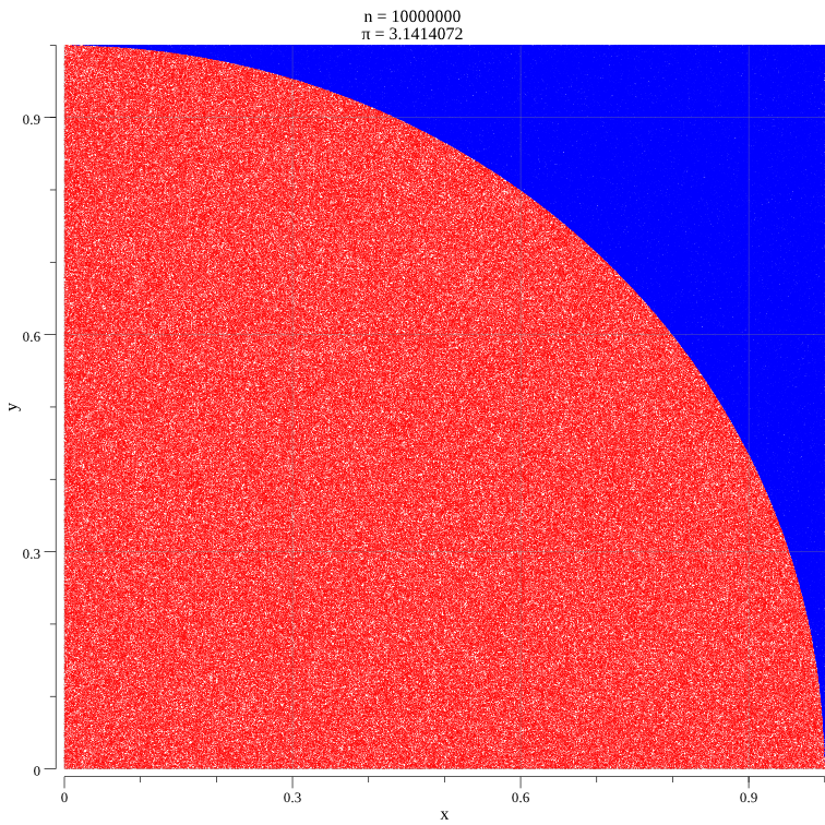
Just for fun, let’s add a little GUI part to visualize where the darts land.
Our GUI will be a web server with two end points:
/will plot a quarter circle inscribed inside the top-right quarter unit square,/datawill send plots over a WebSocket.1 2 3 4 5 6 7 8 9 10 11 12 13 14 15 16 17 18 19 20 21func main() { log.SetPrefix("monte-carlo: ") log.SetFlags(0) n := flag.Int("n", 1e7, "number of samples") flag.Parse() srv := newServer() go srv.pi(*n) http.HandleFunc("/", plotHandle) http.Handle("/data", websocket.Handler(srv.dataHandler)) log.Printf("listening on :8080...") err := http.ListenAndServe(":8080", nil) if err != nil { log.Fatal(err) } }
We will start with creating a web server:
|
|
The in and out fields are slices of (x,y) points that implement the plotter.XYer interface:
1 2 3 4 5 6 7 |
$> go doc gonum.org/v1/plot/plotter.XYs
type XYs []struct{ X, Y float64 }
XYs implements the XYer interface.
func (xys XYs) Len() int
func (xys XYs) XY(i int) (float64, float64) |
1 2 3 4 5 6 7 8 9 |
$> go doc gonum.org/v1/plot/plotter.XYer
type XYer interface {
	// Len returns the number of x, y pairs.
	Len() int

	// XY returns an x, y pair.
	XY(int) (x, y float64)
}
XYer wraps the Len and XY methods. |
The plotter.XYer interface is used by gonum/plot to plot (x,y) points.
Values of type server will be created via the newServer function:
|
|
The run() method is a simple for-loop that listens on the srv.datac channel and sends the resulting plot on the srv.plots channel.
The srv.datac channel is filled in the pi() method:
|
|
|
|
Next is the plot function:
|
|
We create a new hplot.Plot – a thin wrapper around the plot.Plot type from gonum/plot – with the correct labels.
We plot the points inside the circle in red and the ones outside in blue.
The wplot type is just a shim to hold the resulting base64 encoded string of the PNG plot, created with renderImg:
|
|
|
|
At the other end of the srv.plots channel is the dataHandler method that pulls plots out to send them to the web client, over a WebSocket:
|
|
and, finally, the / end point and its home page:
|
|
|
|
Running the Go program and navigating to localhost:8080, you should see:
1 2 |
$> go run ./mc-pi-plot.go monte-carlo: listening on :8080... |

Conclusions
I hope this quick foray into a technique that is at the heart of many physics simulations was fun. The Monte Carlo technique isn’t always the fastest technique to perform simulations (this obviously depends on the “shape” of the function we want to model) but it is deceptively simple, and can be visually “fun” – for some definition of fun.
Note that in this little example, we had fun creating a PNG image, encoding it to JSON+base64 and sending it over a WebSocket.
This was just to exercize a bunch of packages with Go.
Gonum/plot has support for a few backends in addition to PNG: JPEG, TIFF, EPS, PDF, SVG, TeX.
The complete code for mc-pi-plot.go is here.
